2 Getting Started

2.1 The tidyverse

We’ll be using the tidyverse ecosystem of R packages, which are really powerful data science tools that are perfect for these tasks.

We will mainly focus on learning how to use these two libraries:

• dplyr: this is your best friend for transforming and manipulating data (data plyr)

• ggplot2: incredibly robust and modular tool for building visualizations. Provides a lot of flexibility and a rich ecosystem of extensions.

We can install these if we haven’t previously installed them, we can install dplyr using install.packages():

install.packages('dplyr')

And do the same for ggplot2:

install.packages('ggplot2')

We only need to install libraries once on our computer, but any time we start a new R session we need to load the ones we want to use with library(). Let’s go ahead and do that to import the functionality of these functions for the rest of the scripts:

library(dplyr)
library(ggplot2)

2.2 Prepare Data

We have pre-loaded some real query volume data from the QoS subgraph, which shows us query volume ~10 minutes behind real time, compared to on-chain query volume which can take 28 epochs, or never appear on-chain. The latest available data is from 2024-10-18:

Note: you could download a .csv extract of the data above and follow along with every step past this point if you wanted to. This is not the expectation however, and you could only follow-along with this section because the rest of the sections interface with the indexer directly (also for data sources, not only applying operations).

The data provided is already very clean, but we can use the select() function from the dplyr library to select only the columns we care about, and in the order we want to see them in:

select(query_volume, date, subgraph_id, total_query_fees, query_count)

## # A tibble: 236,549 × 4
##    date       subgraph_id                                    total_query_fees query_count
##    <chr>      <chr>                                                     <dbl>       <int>
##  1 2024-10-18 QmUzRg2HHMpbgf6Q4VHKNDbtBEJnyp5JWCh2gUX9AV6jXv            1017.     4393166
##  2 2024-10-18 QmQEYSGSD8t7jTw4gS2dwC4DLvyZceR9fYQ432Ff1hZpCp             787.     3289882
##  3 2024-10-18 QmTZ8ejXJxRo7vDBS4uwqBeGoxLSWbhaA7oXa1RvxunLy7             445.     1926879
##  4 2024-10-18 QmdEz2oUhYGsePUteCGTJWDQZEQ7snGfn7mDMspzn116qa             439.     1913972
##  5 2024-10-18 QmVPCT62C6b2m2D3AnfEF1hJhhmYEenuQtUDLMj1vEBt4m             352.     1533171
##  6 2024-10-18 QmYrEJKHphWBGkqPkEVKSZR9gsoD6RtJs3g3R8iWVhH66Z             302.     1296774
##  7 2024-10-18 Qmbg1qF4YgHjiVfsVt6a13ddrVcRtWyJQfD4LA3CwHM29f             260.     1100999
##  8 2024-10-18 QmdkY9X6Wt3GXA67NYBMJ2NRX6rUsFyQkhk21cqGVZn1sf             194.      849535
##  9 2024-10-18 QmY67iZDTsTdpWXSCotpVPYankwnyHXNT7N95YEn8ccUsn             178.      778428
## 10 2024-10-18 QmTEpd3C2SWgg4YnFDbGHZFLqvUxUZf63fWWjbzkDTsQae             170.      715197
## # ℹ 236,539 more rows

Notice how in the results above the first column is date, and we only kept 4 columns instead of all 8.

Let’s overwrite the existing query_volume dataset by specifying as = to the previous result:

query_volume = select(query_volume, date, subgraph_id, total_query_fees, query_count)

2.2.1 Filter Data

Nice! Next up, let’s work towards visualizing the query volume of a particular subgraph 📈. The first thing we want to do is filter our data to one specific subgraph deployment, and save the results in a new dataset we can use for the visualization. This time we can use the filter() function, which is still from dplyr, to only return rows that match a specific condition.

On the original data query_volume, we can apply the filter() function, and only match rows where the subgraph_id is QmUzRg2HHMpbgf6Q4VHKNDbtBEJnyp5JWCh2gUX9AV6jXv:

# start with the data
query_volume %>% 
  # filter to rows matching a specific subgraph_id
  filter(subgraph_id == 'QmUzRg2HHMpbgf6Q4VHKNDbtBEJnyp5JWCh2gUX9AV6jXv')

## # A tibble: 28 × 4
##    date       subgraph_id                                    total_query_fees query_count
##    <chr>      <chr>                                                     <dbl>       <int>
##  1 2024-10-18 QmUzRg2HHMpbgf6Q4VHKNDbtBEJnyp5JWCh2gUX9AV6jXv            1017.     4393166
##  2 2024-10-17 QmUzRg2HHMpbgf6Q4VHKNDbtBEJnyp5JWCh2gUX9AV6jXv            1080.     4675752
##  3 2024-10-16 QmUzRg2HHMpbgf6Q4VHKNDbtBEJnyp5JWCh2gUX9AV6jXv            1086.     4722228
##  4 2024-10-15 QmUzRg2HHMpbgf6Q4VHKNDbtBEJnyp5JWCh2gUX9AV6jXv             397.     1751990
##  5 2024-10-14 QmUzRg2HHMpbgf6Q4VHKNDbtBEJnyp5JWCh2gUX9AV6jXv             992.     4343594
##  6 2024-10-13 QmUzRg2HHMpbgf6Q4VHKNDbtBEJnyp5JWCh2gUX9AV6jXv            1014.     4284406
##  7 2024-10-12 QmUzRg2HHMpbgf6Q4VHKNDbtBEJnyp5JWCh2gUX9AV6jXv             936.     3988545
##  8 2024-10-11 QmUzRg2HHMpbgf6Q4VHKNDbtBEJnyp5JWCh2gUX9AV6jXv            1041.     4381377
##  9 2024-10-10 QmUzRg2HHMpbgf6Q4VHKNDbtBEJnyp5JWCh2gUX9AV6jXv             805.     3342601
## 10 2024-10-09 QmUzRg2HHMpbgf6Q4VHKNDbtBEJnyp5JWCh2gUX9AV6jXv             642.     2656546
## # ℹ 18 more rows

In the command above, we checked for subgraph_id matching the value using ==. This produced a value of True/False for each row, and only gave back rows where the match was True. We use == because = is reserved for assigning things.

Here we use a “pipe operator” (%>%), which lets us start with our dataset, and clearly apply one operation at a time like the code above. That is all you need to conceptually understand, but make sure you understand what action we are taking in the example above. You can read more about the pipe operator in this concise bonus section example at the bottom of this page.

Let’s run the same exact code as the above, but add subgraph_data = to the start, to save the new results to a new dataset we are creating subgraph_data:

# start with query_volume, filter to subgraph, assign results to new data "query_volume"
subgraph_data = query_volume %>% 
  # filter to rows matching a specific subgraph_id
  filter(subgraph_id == 'QmUzRg2HHMpbgf6Q4VHKNDbtBEJnyp5JWCh2gUX9AV6jXv')

Now we can view the new data which was filtered to the specific subgraph:

subgraph_data

## # A tibble: 28 × 4
##    date       subgraph_id                                    total_query_fees query_count
##    <chr>      <chr>                                                     <dbl>       <int>
##  1 2024-10-18 QmUzRg2HHMpbgf6Q4VHKNDbtBEJnyp5JWCh2gUX9AV6jXv            1017.     4393166
##  2 2024-10-17 QmUzRg2HHMpbgf6Q4VHKNDbtBEJnyp5JWCh2gUX9AV6jXv            1080.     4675752
##  3 2024-10-16 QmUzRg2HHMpbgf6Q4VHKNDbtBEJnyp5JWCh2gUX9AV6jXv            1086.     4722228
##  4 2024-10-15 QmUzRg2HHMpbgf6Q4VHKNDbtBEJnyp5JWCh2gUX9AV6jXv             397.     1751990
##  5 2024-10-14 QmUzRg2HHMpbgf6Q4VHKNDbtBEJnyp5JWCh2gUX9AV6jXv             992.     4343594
##  6 2024-10-13 QmUzRg2HHMpbgf6Q4VHKNDbtBEJnyp5JWCh2gUX9AV6jXv            1014.     4284406
##  7 2024-10-12 QmUzRg2HHMpbgf6Q4VHKNDbtBEJnyp5JWCh2gUX9AV6jXv             936.     3988545
##  8 2024-10-11 QmUzRg2HHMpbgf6Q4VHKNDbtBEJnyp5JWCh2gUX9AV6jXv            1041.     4381377
##  9 2024-10-10 QmUzRg2HHMpbgf6Q4VHKNDbtBEJnyp5JWCh2gUX9AV6jXv             805.     3342601
## 10 2024-10-09 QmUzRg2HHMpbgf6Q4VHKNDbtBEJnyp5JWCh2gUX9AV6jXv             642.     2656546
## # ℹ 18 more rows

R only does exactly what you ask it to do. So when we just execute subgraph_data, this simply returns the unchanged/current dataset or R object. If we apply filter or other operations and don’t assign the result to a new variable with =, we will see the results of the data with the transformations applied. If we then stored those results in a new dataset, it would no longer print the results until we asked it for the new data.

From this point forward we won’t keep showing the code that just prints the new data as it doesn’t add new material information and makes the tutorial more concise.

2.2.2 Mutate/Transform

This is looking pretty good! The only thing we still need to fix is the date which has a character data type, and we want to convert to a Date type to make our life easier in later steps. To do this, we can use the mutate() function to apply a transformation on the date column of the data. We will simply use as.Date() to convert the column, and overwrite the same column:

subgraph_data %<>% 
  # convert to date
  mutate(date = as.Date(date))

## # A tibble: 28 × 4
##    date       subgraph_id                                    total_query_fees query_count
##    <date>     <chr>                                                     <dbl>       <int>
##  1 2024-10-18 QmUzRg2HHMpbgf6Q4VHKNDbtBEJnyp5JWCh2gUX9AV6jXv            1017.     4393166
##  2 2024-10-17 QmUzRg2HHMpbgf6Q4VHKNDbtBEJnyp5JWCh2gUX9AV6jXv            1080.     4675752
##  3 2024-10-16 QmUzRg2HHMpbgf6Q4VHKNDbtBEJnyp5JWCh2gUX9AV6jXv            1086.     4722228
##  4 2024-10-15 QmUzRg2HHMpbgf6Q4VHKNDbtBEJnyp5JWCh2gUX9AV6jXv             397.     1751990
##  5 2024-10-14 QmUzRg2HHMpbgf6Q4VHKNDbtBEJnyp5JWCh2gUX9AV6jXv             992.     4343594
##  6 2024-10-13 QmUzRg2HHMpbgf6Q4VHKNDbtBEJnyp5JWCh2gUX9AV6jXv            1014.     4284406
##  7 2024-10-12 QmUzRg2HHMpbgf6Q4VHKNDbtBEJnyp5JWCh2gUX9AV6jXv             936.     3988545
##  8 2024-10-11 QmUzRg2HHMpbgf6Q4VHKNDbtBEJnyp5JWCh2gUX9AV6jXv            1041.     4381377
##  9 2024-10-10 QmUzRg2HHMpbgf6Q4VHKNDbtBEJnyp5JWCh2gUX9AV6jXv             805.     3342601
## 10 2024-10-09 QmUzRg2HHMpbgf6Q4VHKNDbtBEJnyp5JWCh2gUX9AV6jXv             642.     2656546
## # ℹ 18 more rows

2.3 Visualize Results

Next we will start using functions from ggplot2 to start visualizing data. We already imported this library earlier, so we can go ahead and start using ggplot() and related functions.

Our starting point is always our data, so we start with: subgraph_data %>%

Then, we want to map the chart to the correct x and y variables. We can use aes() which stands for aesthetics, and map the x variable to date, and y to query_count, which will give us a visualization of query count over time:

subgraph_data %>% 
  # set ggplot mappings
  ggplot(aes(x=date, y=query_count))

But wait - what about the actual visualization?

We only established what should be on the x and y axis, but we didn’t specify what we actually want to visualize. Let’s go ahead and add a point for each observation by adding another layer to the chart with geom_point():

subgraph_data %>% 
  # set ggplot mappings
  ggplot(aes(x=date, y=query_count)) +
  # add actual points to the chart
  geom_point()

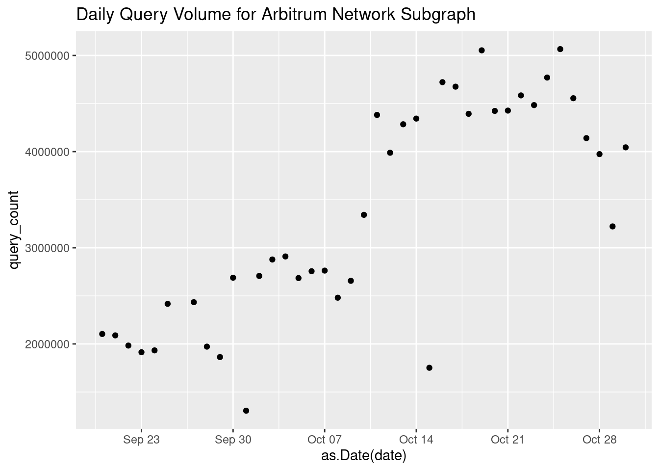
In more complex examples we can map additional layers to different things, but in this case by just adding geom_point() ggplot already understands what we want because we told it which variables we want on x and y axis, and what we want to visualize those observations as.

Within the ggplot usage, we use + which is conceptually the same as %>% to make changes to the plot. We use %>% when we start with an R object, but use + to add new layers to a chart in ggplot.

We can save the current chart in subgraph_chart, and keep adding new changes from this point:

subgraph_chart = subgraph_data %>% 
  # set ggplot mappings
  ggplot(aes(x=as.Date(date), y=query_count)) +
  # create a line
  geom_point()

Now we can make changes to subgraph_chart, for example we can add a title with ggtitle()

subgraph_chart + ggtitle('Daily Query Volume for Arbitrum Network Subgraph')

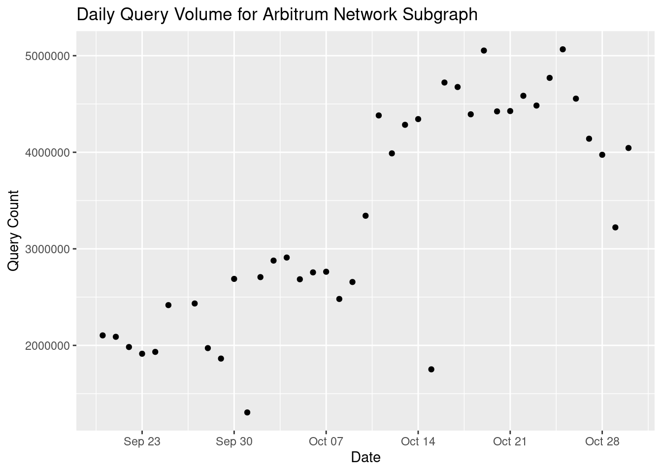
Let’s add the title like above with ggtitle, and also add xlab() and ylab() to change the x and y axis labels.

subgraph_chart = subgraph_chart + 
  # add title
  ggtitle('Daily Query Volume for Arbitrum Network Subgraph') +
  # change x-axis label
  xlab('Date') +
  # change y-axis label
  ylab('Query Count')

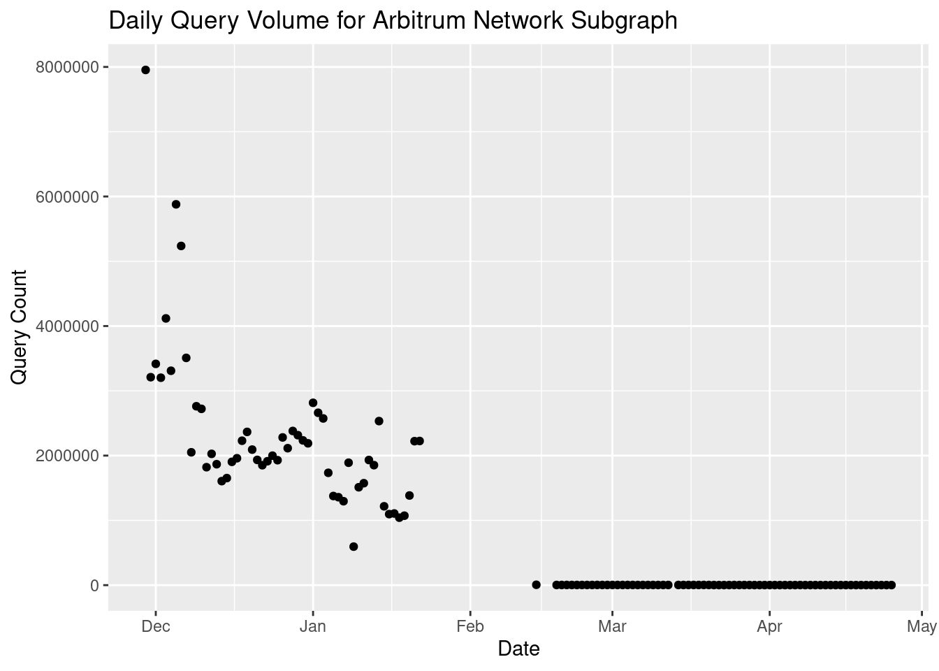
Let’s make the numbers on the y-axis more readable by adding commas. We will use scale_y_continuous() and specify the labels as comma. comma is an extension outside of the base ggplot2 library, so we first do library(scales) to import what we need:

library(scales)
subgraph_chart = subgraph_chart + scale_y_continuous(labels = comma)

# View modified chart
subgraph_chart

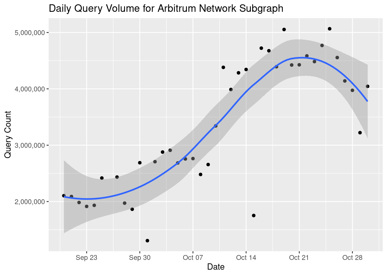
Nice! From this point there are a number of cool things we can do. Let’s start by taking the chart we have, and making it interactive. To do this, let’s import the plotly library, and simply wrap our chart in ggplotly():

library(plotly)
# wrap chart in command that makes it interactive
ggplotly(subgraph_chart)

The above maintained our chart, but you can now hover over the data points and view their precise values.

We can do a bunch of other things. We can add a line showing the trend over time adding stat_smooth() to the chart:

subgraph_chart + stat_smooth()

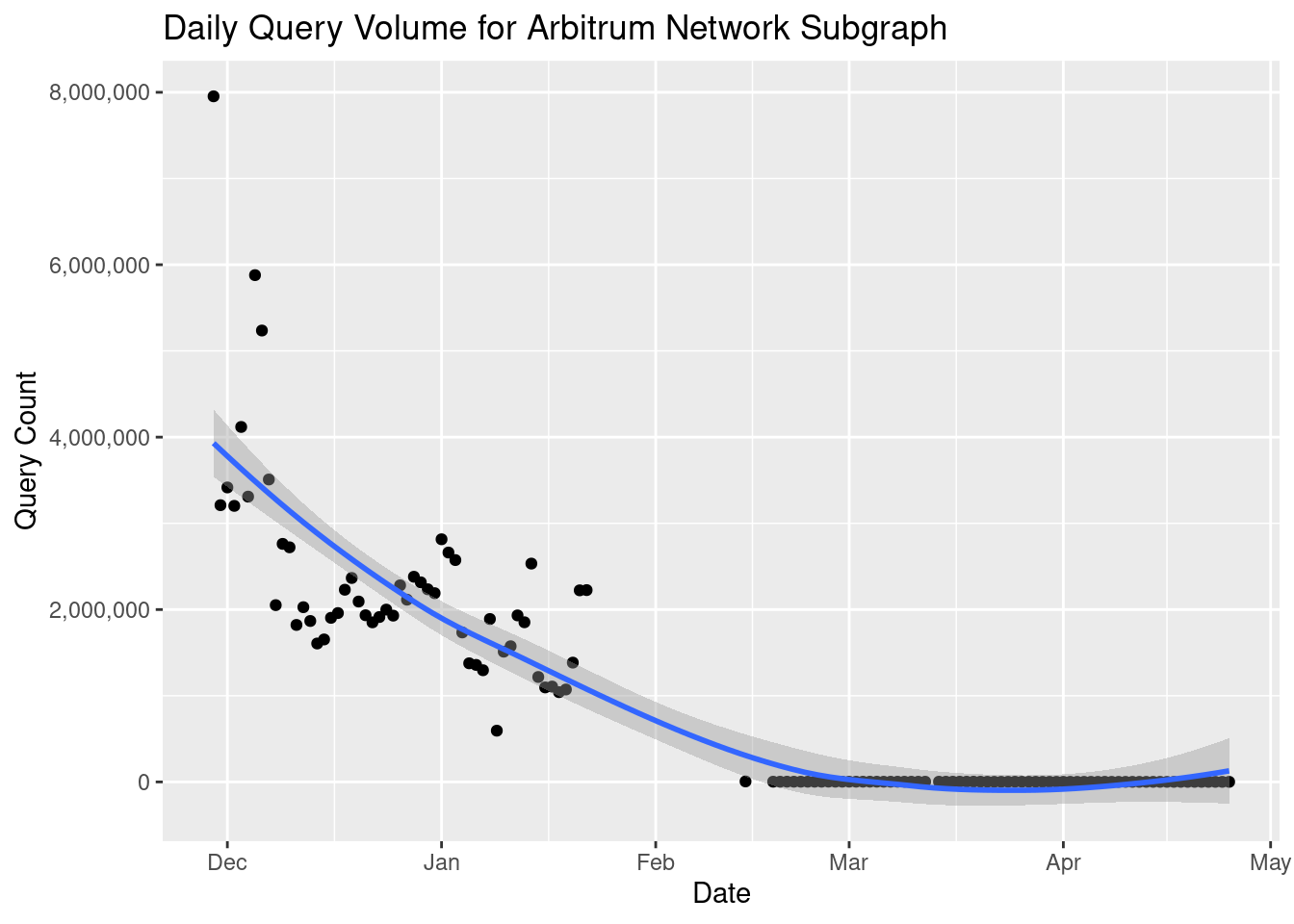
Or a linear regression line:

# Add linear regression line
subgraph_chart + stat_smooth(method = 'lm', color='red')

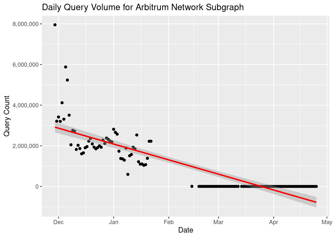
We will get more sophisticated with this in a second when we produce a forecast. For now, let’s keep improving the look of the chart.

Let’s bring in the ggthemes extension, and apply a theme using theme_economist():

library(ggthemes)
# apply theme
subgraph_chart = subgraph_chart + theme_economist()
# view chart with theme applied
subgraph_chart

Next, let’s label the high and low points in the data using the ggforce library. We will use geom_mark_ellipse() to circle the point matching the highest point shown, and another one to circle the lowest one:

library(ggforce)
# Create a data frame for the annotation
annotation_data = subgraph_data %>%
  filter(query_count == max(query_count) | query_count == min(query_count)) %>%
  mutate(label = format(date, "%Y-%m-%d"),
         description = ifelse(query_count == max(query_count),
                              paste0('Highest query volume day had ', query_count, ' queries'),
                              paste0('Lowest query volume day had ', query_count, ' queries')))

# Add the annotation to the chart
subgraph_chart = subgraph_chart +
  geom_mark_ellipse(data = annotation_data,
                    aes(label = label, description = description))

# View the modified chart
subgraph_chart

2.3.1 Add Forecast

We will use the prophet library, released by facebook research. This library is very easy to use, and does a good job with time-series forecasting that works out of the box by intelligently adapting parameters based on the data it sees.

library(prophet)

The library requires the data to be formatted with only two columns, one with the date, and one with the variable we want to predict, in our case query_count. So as a first step we will rename date to ds, and query_count to y:

prophet_data = subgraph_data %>%
  select(ds = date, y = query_count)

Now we can create and fit the model to the data:

m = prophet(prophet_data)

## $growth
## [1] "linear"
## 
## $changepoints
##  [1] "2024-09-21 GMT" "2024-09-22 GMT" "2024-09-23 GMT" "2024-09-24 GMT" "2024-09-25 GMT" "2024-09-27 GMT" "2024-09-28 GMT"
##  [8] "2024-09-29 GMT" "2024-09-30 GMT" "2024-10-01 GMT" "2024-10-02 GMT" "2024-10-03 GMT" "2024-10-04 GMT" "2024-10-05 GMT"
## [15] "2024-10-06 GMT" "2024-10-07 GMT" "2024-10-08 GMT" "2024-10-09 GMT" "2024-10-10 GMT" "2024-10-11 GMT" "2024-10-12 GMT"
## 
## $n.changepoints
## [1] 21
## 
## $changepoint.range
## [1] 0.8
## 
## $yearly.seasonality
## [1] "auto"
## 
## $weekly.seasonality
## [1] "auto"
## 
## $daily.seasonality
## [1] "auto"
## 
## $holidays
## NULL
## 
## $seasonality.mode
## [1] "additive"
## 
## $seasonality.prior.scale
## [1] 10
## 
## $changepoint.prior.scale
## [1] 0.05
## 
## $holidays.prior.scale
## [1] 10
## 
## $mcmc.samples
## [1] 0
## 
## $interval.width
## [1] 0.8
## 
## $uncertainty.samples
## [1] 1000
## 
## $specified.changepoints
## [1] FALSE
## 
## $start
## [1] "2024-09-20 GMT"
## 
## $y.scale
## [1] 4722228
## 
## $logistic.floor
## [1] FALSE
## 
## $t.scale
## [1] 2419200
## 
## $changepoints.t
##  [1] 0.03571429 0.07142857 0.10714286 0.14285714 0.17857143 0.25000000 0.28571429 0.32142857 0.35714286 0.39285714 0.42857143
## [12] 0.46428571 0.50000000 0.53571429 0.57142857 0.60714286 0.64285714 0.67857143 0.71428571 0.75000000 0.78571429
## 
## $seasonalities
## $seasonalities$weekly
## $seasonalities$weekly$period
## [1] 7
## 
## $seasonalities$weekly$fourier.order
## [1] 3
## 
## $seasonalities$weekly$prior.scale
## [1] 10
## 
## $seasonalities$weekly$mode
## [1] "additive"
## 
## $seasonalities$weekly$condition.name
## NULL
## 
## 
## 
## $extra_regressors
## list()
## 
## $country_holidays
## NULL
## 
## $stan.fit
## $stan.fit$par
## $stan.fit$par$k
## [1] 0.5232871
## 
## $stan.fit$par$m
## [1] 0.3401971
## 
## $stan.fit$par$delta
##  [1]  0.000000000337106107  0.000000000238590393  0.000000000376850848 -0.000000000134645112  0.000000000351068902
##  [6] -0.000000000035334454  0.000000000122208725  0.000000000282528017  0.000000000216758213  0.000000000102925676
## [11]  0.000000203224932728  0.000000000534541393 -0.000000000001102959  0.000000000495001327 -0.000000000201630005
## [16]  0.000000149487334663  0.000000000118532194  0.000000000354272190 -0.000000000010725153 -0.000000000197387628
## [21]  0.000000000081128372
## 
## $stan.fit$par$sigma_obs
## [1] 0.09736997
## 
## $stan.fit$par$beta
## [1]  0.072552145  0.041831357 -0.008025221  0.065790424 -0.051444360 -0.052391591
## 
## $stan.fit$par$trend
##  [1] 0.3401971 0.3588860 0.3775748 0.3962636 0.4149524 0.4336413 0.4710189 0.4897077 0.5083965 0.5270854 0.5457742 0.5644630
## [13] 0.5831519 0.6018407 0.6205295 0.6392183 0.6579072 0.6765960 0.6952849 0.7139737 0.7326625 0.7513514 0.7700402 0.7887290
## [25] 0.8074179 0.8261067 0.8447955 0.8634844
## 
## 
## $stan.fit$value
## [1] 51.32611
## 
## $stan.fit$return_code
## [1] 0
## 
## $stan.fit$theta_tilde
##              k         m           delta[1]           delta[2]           delta[3]            delta[4]           delta[5]
## [1,] 0.5232871 0.3401971 0.0000000003371061 0.0000000002385904 0.0000000003768508 -0.0000000001346451 0.0000000003510689
##                  delta[6]           delta[7]          delta[8]           delta[9]          delta[10]       delta[11]
## [1,] -0.00000000003533445 0.0000000001222087 0.000000000282528 0.0000000002167582 0.0000000001029257 0.0000002032249
##               delta[12]             delta[13]          delta[14]         delta[15]       delta[16]          delta[17]
## [1,] 0.0000000005345414 -0.000000000001102959 0.0000000004950013 -0.00000000020163 0.0000001494873 0.0000000001185322
##               delta[18]            delta[19]           delta[20]           delta[21]  sigma_obs    beta[1]    beta[2]
## [1,] 0.0000000003542722 -0.00000000001072515 -0.0000000001973876 0.00000000008112837 0.09736997 0.07255214 0.04183136
##           beta[3]    beta[4]     beta[5]     beta[6]  trend[1] trend[2]  trend[3]  trend[4]  trend[5]  trend[6]  trend[7]
## [1,] -0.008025221 0.06579042 -0.05144436 -0.05239159 0.3401971 0.358886 0.3775748 0.3962636 0.4149524 0.4336413 0.4710189
##       trend[8]  trend[9] trend[10] trend[11] trend[12] trend[13] trend[14] trend[15] trend[16] trend[17] trend[18] trend[19]
## [1,] 0.4897077 0.5083965 0.5270854 0.5457742  0.564463 0.5831519 0.6018407 0.6205295 0.6392183 0.6579072  0.676596 0.6952849
##      trend[20] trend[21] trend[22] trend[23] trend[24] trend[25] trend[26] trend[27] trend[28]
## [1,] 0.7139737 0.7326625 0.7513514 0.7700402  0.788729 0.8074179 0.8261067 0.8447955 0.8634844
## 
## 
## $params
## $params$k
## [1] 0.5232871
## 
## $params$m
## [1] 0.3401971
## 
## $params$delta
##                    [,1]               [,2]               [,3]                [,4]               [,5]                 [,6]
## [1,] 0.0000000003371061 0.0000000002385904 0.0000000003768508 -0.0000000001346451 0.0000000003510689 -0.00000000003533445
##                    [,7]              [,8]               [,9]              [,10]           [,11]              [,12]
## [1,] 0.0000000001222087 0.000000000282528 0.0000000002167582 0.0000000001029257 0.0000002032249 0.0000000005345414
##                      [,13]              [,14]             [,15]           [,16]              [,17]              [,18]
## [1,] -0.000000000001102959 0.0000000004950013 -0.00000000020163 0.0000001494873 0.0000000001185322 0.0000000003542722
##                     [,19]               [,20]               [,21]
## [1,] -0.00000000001072515 -0.0000000001973876 0.00000000008112837
## 
## $params$sigma_obs
## [1] 0.09736997
## 
## $params$beta
##            [,1]       [,2]         [,3]       [,4]        [,5]        [,6]
## [1,] 0.07255214 0.04183136 -0.008025221 0.06579042 -0.05144436 -0.05239159
## 
## $params$trend
##  [1] 0.3401971 0.3588860 0.3775748 0.3962636 0.4149524 0.4336413 0.4710189 0.4897077 0.5083965 0.5270854 0.5457742 0.5644630
## [13] 0.5831519 0.6018407 0.6205295 0.6392183 0.6579072 0.6765960 0.6952849 0.7139737 0.7326625 0.7513514 0.7700402 0.7887290
## [25] 0.8074179 0.8261067 0.8447955 0.8634844
## 
## 
## $history
## # A tibble: 28 × 5
##    ds                        y floor      t y_scaled
##    <dttm>                <dbl> <dbl>  <dbl>    <dbl>
##  1 2024-09-20 00:00:00 2103572     0 0         0.445
##  2 2024-09-21 00:00:00 2088898     0 0.0357    0.442
##  3 2024-09-22 00:00:00 1983096     0 0.0714    0.420
##  4 2024-09-23 00:00:00 1913592     0 0.107     0.405
##  5 2024-09-24 00:00:00 1932800     0 0.143     0.409
##  6 2024-09-25 00:00:00 2417032     0 0.179     0.512
##  7 2024-09-27 00:00:00 2433971     0 0.25      0.515
##  8 2024-09-28 00:00:00 1971945     0 0.286     0.418
##  9 2024-09-29 00:00:00 1863463     0 0.321     0.395
## 10 2024-09-30 00:00:00 2688731     0 0.357     0.569
## # ℹ 18 more rows
## 
## $history.dates
##  [1] "2024-09-20 GMT" "2024-09-21 GMT" "2024-09-22 GMT" "2024-09-23 GMT" "2024-09-24 GMT" "2024-09-25 GMT" "2024-09-27 GMT"
##  [8] "2024-09-28 GMT" "2024-09-29 GMT" "2024-09-30 GMT" "2024-10-01 GMT" "2024-10-02 GMT" "2024-10-03 GMT" "2024-10-04 GMT"
## [15] "2024-10-05 GMT" "2024-10-06 GMT" "2024-10-07 GMT" "2024-10-08 GMT" "2024-10-09 GMT" "2024-10-10 GMT" "2024-10-11 GMT"
## [22] "2024-10-12 GMT" "2024-10-13 GMT" "2024-10-14 GMT" "2024-10-15 GMT" "2024-10-16 GMT" "2024-10-17 GMT" "2024-10-18 GMT"
## 
## $train.holiday.names
## NULL
## 
## $train.component.cols
##   additive_terms weekly multiplicative_terms
## 1              1      1                    0
## 2              1      1                    0
## 3              1      1                    0
## 4              1      1                    0
## 5              1      1                    0
## 6              1      1                    0
## 
## $component.modes
## $component.modes$additive
## [1] "weekly"                    "additive_terms"            "extra_regressors_additive" "holidays"                 
## 
## $component.modes$multiplicative
## [1] "multiplicative_terms"            "extra_regressors_multiplicative"
## 
## 
## $fit.kwargs
## list()
## 
## attr(,"class")
## [1] "prophet" "list"

Next we construct a dataset that’s 30 days into the future to make the forecasts for:

future = make_future_dataframe(m, periods = 30)

Next we can make the forecast:

forecast = predict(m, future)

Now we can plot the results:

plot(m, forecast)

2.4 Summarize Data

Let’s do something similar (minus the forecast), but let’s aggregate the results across all subgraphs. Here is the raw data again as a reminder:

## # A tibble: 236,549 × 4
##    date       subgraph_id                                    total_query_fees query_count
##    <chr>      <chr>                                                     <dbl>       <int>
##  1 2024-10-18 QmUzRg2HHMpbgf6Q4VHKNDbtBEJnyp5JWCh2gUX9AV6jXv            1017.     4393166
##  2 2024-10-18 QmQEYSGSD8t7jTw4gS2dwC4DLvyZceR9fYQ432Ff1hZpCp             787.     3289882
##  3 2024-10-18 QmTZ8ejXJxRo7vDBS4uwqBeGoxLSWbhaA7oXa1RvxunLy7             445.     1926879
##  4 2024-10-18 QmdEz2oUhYGsePUteCGTJWDQZEQ7snGfn7mDMspzn116qa             439.     1913972
##  5 2024-10-18 QmVPCT62C6b2m2D3AnfEF1hJhhmYEenuQtUDLMj1vEBt4m             352.     1533171
##  6 2024-10-18 QmYrEJKHphWBGkqPkEVKSZR9gsoD6RtJs3g3R8iWVhH66Z             302.     1296774
##  7 2024-10-18 Qmbg1qF4YgHjiVfsVt6a13ddrVcRtWyJQfD4LA3CwHM29f             260.     1100999
##  8 2024-10-18 QmdkY9X6Wt3GXA67NYBMJ2NRX6rUsFyQkhk21cqGVZn1sf             194.      849535
##  9 2024-10-18 QmY67iZDTsTdpWXSCotpVPYankwnyHXNT7N95YEn8ccUsn             178.      778428
## 10 2024-10-18 QmTEpd3C2SWgg4YnFDbGHZFLqvUxUZf63fWWjbzkDTsQae             170.      715197
## # ℹ 236,539 more rows

We can first group_by() date, and then summarize() the sum of total_query_fees by day, and save the results in daily_summary:

daily_summary = query_volume %>% 
  # group by date
  group_by(date) %>% 
  # summarize query fees by date
  summarize(total_query_fees = sum(total_query_fees))

# view new summarized data
daily_summary

## # A tibble: 29 × 2
##    date       total_query_fees
##    <chr>                 <dbl>
##  1 2024-09-20           10287.
##  2 2024-09-21            9918.
##  3 2024-09-22            8282.
##  4 2024-09-23           12813.
##  5 2024-09-24           14213.
##  6 2024-09-25           16328.
##  7 2024-09-26            3758.
##  8 2024-09-27           18133.
##  9 2024-09-28           11875.
## 10 2024-09-29           11049.
## # ℹ 19 more rows

Now we can visualize these results:

daily_summary_chart = daily_summary %>%
  # set ggplot mappings
  ggplot(aes(x = as.Date(date), y = total_query_fees)) +
  # create a line
  geom_line() +
  # add title
  ggtitle('Query Fees on The Graph Decentralized Network') +
  # change x-axis label
  xlab('Date') +
  # change y-axis label
  ylab('Query Fees (GRT)') +
  # adjust y-axis to show commas thousand separator
  scale_y_continuous(labels = comma) +
  # apply theme
  theme_economist()

2.5 Pulling Data

This section started with already pulled data to focus on teaching you what you need to know to understand the code in the next sections. But what if you wanted to pull data from a GraphQL endpoint yourself? That’s exactly what the next section begins with, and you can move on.

You will walk through the first iteration of Ricky’s indexer automated allocation management, and how it actually works step by step.

2.6 Bonus learning: pipe operator explanation

The real magic of the tidyverse comes from creating a separation between the data, and the operations that get applied. One of the main tools it accomplishes with, is the pipe operator, which is explained below.

Let’s take this example where we apply a select() and arrange() transformation correctly, but without the pipe operator:

arrange(select(query_volume, date, subgraph_id, total_query_fees, query_count), desc(date), desc(total_query_fees))

## # A tibble: 236,549 × 4
##    date       subgraph_id                                    total_query_fees query_count
##    <chr>      <chr>                                                     <dbl>       <int>
##  1 2024-10-18 QmUzRg2HHMpbgf6Q4VHKNDbtBEJnyp5JWCh2gUX9AV6jXv            1017.     4393166
##  2 2024-10-18 QmQEYSGSD8t7jTw4gS2dwC4DLvyZceR9fYQ432Ff1hZpCp             787.     3289882
##  3 2024-10-18 QmTZ8ejXJxRo7vDBS4uwqBeGoxLSWbhaA7oXa1RvxunLy7             445.     1926879
##  4 2024-10-18 QmdEz2oUhYGsePUteCGTJWDQZEQ7snGfn7mDMspzn116qa             439.     1913972
##  5 2024-10-18 QmVPCT62C6b2m2D3AnfEF1hJhhmYEenuQtUDLMj1vEBt4m             352.     1533171
##  6 2024-10-18 QmYrEJKHphWBGkqPkEVKSZR9gsoD6RtJs3g3R8iWVhH66Z             302.     1296774
##  7 2024-10-18 Qmbg1qF4YgHjiVfsVt6a13ddrVcRtWyJQfD4LA3CwHM29f             260.     1100999
##  8 2024-10-18 QmdkY9X6Wt3GXA67NYBMJ2NRX6rUsFyQkhk21cqGVZn1sf             194.      849535
##  9 2024-10-18 QmY67iZDTsTdpWXSCotpVPYankwnyHXNT7N95YEn8ccUsn             178.      778428
## 10 2024-10-18 QmTEpd3C2SWgg4YnFDbGHZFLqvUxUZf63fWWjbzkDTsQae             170.      715197
## # ℹ 236,539 more rows

In the example above it becomes really hard to keep track of what data we are starting with, and what operations are being applied. Pipes are a powerful tool for clearly expressing a sequence of multiple operations. Here we start with our dataset, then we “pipe” (%>% operator) each operation one step at a time in a way that is very logically ordered and easy to read:

# start with the data
query_volume %>%
  # select the columns we want to keep
  select(date, subgraph_id, total_query_fees, query_count) %>%
  # order the rows by the latest dates, and highest query counts
  arrange(desc(date), desc(total_query_fees))

## # A tibble: 236,549 × 4
##    date       subgraph_id                                    total_query_fees query_count
##    <chr>      <chr>                                                     <dbl>       <int>
##  1 2024-10-18 QmUzRg2HHMpbgf6Q4VHKNDbtBEJnyp5JWCh2gUX9AV6jXv            1017.     4393166
##  2 2024-10-18 QmQEYSGSD8t7jTw4gS2dwC4DLvyZceR9fYQ432Ff1hZpCp             787.     3289882
##  3 2024-10-18 QmTZ8ejXJxRo7vDBS4uwqBeGoxLSWbhaA7oXa1RvxunLy7             445.     1926879
##  4 2024-10-18 QmdEz2oUhYGsePUteCGTJWDQZEQ7snGfn7mDMspzn116qa             439.     1913972
##  5 2024-10-18 QmVPCT62C6b2m2D3AnfEF1hJhhmYEenuQtUDLMj1vEBt4m             352.     1533171
##  6 2024-10-18 QmYrEJKHphWBGkqPkEVKSZR9gsoD6RtJs3g3R8iWVhH66Z             302.     1296774
##  7 2024-10-18 Qmbg1qF4YgHjiVfsVt6a13ddrVcRtWyJQfD4LA3CwHM29f             260.     1100999
##  8 2024-10-18 QmdkY9X6Wt3GXA67NYBMJ2NRX6rUsFyQkhk21cqGVZn1sf             194.      849535
##  9 2024-10-18 QmY67iZDTsTdpWXSCotpVPYankwnyHXNT7N95YEn8ccUsn             178.      778428
## 10 2024-10-18 QmTEpd3C2SWgg4YnFDbGHZFLqvUxUZf63fWWjbzkDTsQae             170.      715197
## # ℹ 236,539 more rows

The command above shows us the results with the transformations applied, but we did not yet overwrite the original query_volume data:

query_volume

## # A tibble: 236,549 × 4
##    date       subgraph_id                                    total_query_fees query_count
##    <chr>      <chr>                                                     <dbl>       <int>
##  1 2024-10-18 QmUzRg2HHMpbgf6Q4VHKNDbtBEJnyp5JWCh2gUX9AV6jXv            1017.     4393166
##  2 2024-10-18 QmQEYSGSD8t7jTw4gS2dwC4DLvyZceR9fYQ432Ff1hZpCp             787.     3289882
##  3 2024-10-18 QmTZ8ejXJxRo7vDBS4uwqBeGoxLSWbhaA7oXa1RvxunLy7             445.     1926879
##  4 2024-10-18 QmdEz2oUhYGsePUteCGTJWDQZEQ7snGfn7mDMspzn116qa             439.     1913972
##  5 2024-10-18 QmVPCT62C6b2m2D3AnfEF1hJhhmYEenuQtUDLMj1vEBt4m             352.     1533171
##  6 2024-10-18 QmYrEJKHphWBGkqPkEVKSZR9gsoD6RtJs3g3R8iWVhH66Z             302.     1296774
##  7 2024-10-18 Qmbg1qF4YgHjiVfsVt6a13ddrVcRtWyJQfD4LA3CwHM29f             260.     1100999
##  8 2024-10-18 QmdkY9X6Wt3GXA67NYBMJ2NRX6rUsFyQkhk21cqGVZn1sf             194.      849535
##  9 2024-10-18 QmY67iZDTsTdpWXSCotpVPYankwnyHXNT7N95YEn8ccUsn             178.      778428
## 10 2024-10-18 QmTEpd3C2SWgg4YnFDbGHZFLqvUxUZf63fWWjbzkDTsQae             170.      715197
## # ℹ 236,539 more rows

By running the same exact command as before, but modifying the first pipe to be %<>% instead of %>%, we can overwrite the query_volume data with the transformations:

# start with the data
query_volume %<>%
  # select the columns we want to keep
  select(date, subgraph_id, total_query_fees, query_count) %>%
  # order the rows by the latest dates, and highest query counts
  arrange(desc(date), desc(total_query_fees))

Nice job! Now you have everything that you need to conceptually follow-along with each step. Let’s jump right in and start by closing our active allocations